Single Model Performance Index (SMPI)

Overview

This diagnostic calculates the Single Model Performance Index (SMPI) following Reichler and Kim (2008). The SMPI (called “I²”) is based on the comparison of several different climate variables (atmospheric, surface and oceanic) between climate model simulations and observations or reanalyses, and it focuses on the validation of the time-mean state of climate. For I² to be determined, the differences between the climatological mean of each model variable and observations at each of the available data grid points are calculated, and scaled to the interannual variance from the validating observations. This interannual variability is determined by performing a bootstrapping method (random selection with replacement) for the creation of a large synthetic ensemble of observational climatologies. The results are then scaled to the average error from a reference ensemble of models, and in a final step the mean over all climate variables and one model is calculated. The plot shows the I² values for each model (orange circles) and the multi-model mean (black circle), with the diameter of each circle representing the range of I² values encompassed by the 5th and 95th percentiles of the bootstrap ensemble. The I² values vary around one, with values greater than one for underperforming models, and values less than one for more accurate models.

Note: The SMPI diagnostic needs all indicated variables from all added models for exactly the same time period to be calculated correctly. If one model does not provide a specific variable, either that model cannot be added to the SMPI calculations, or the missing variable has to be removed from the diagnostics all together.

Available recipes and diagnostics

Recipes are stored in recipes/

• recipe_smpi.yml

• recipe_smpi_4cds.yml

Diagnostics are stored in diag_scripts/perfmetrics/

• main.ncl: calculates and (optionally) plots annual/seasonal cycles, zonal means, lat-lon fields and time-lat-lon fields. The calculated fields can also be plotted as difference w.r.t. a given reference dataset. main.ncl also calculates RMSD, bias and taylor metrics. Input data have to be regridded to a common grid in the preprocessor. Each plot type is created by a separated routine, as detailed below.

• cycle_zonal.ncl: calculates single model performance index (Reichler and Kim, 2008). It requires fields precalculated by main.ncl.

• collect.ncl: collects the metrics previously calculated by cycle_latlon.ncl and passes them to the plotting functions.

User settings

1. perfmetrics/main.ncl

   Required settings for script

   • plot_type: only “cycle_latlon (time, lat, lon)” and “cycle_zonal (time, plev, lat)” available for SMPI; usage is defined in the recipe and is dependent on the used variable (2D variable: cycle_latlon, 3D variable: cycle_zonal)

   • time_avg: type of time average (only “yearly” allowed for SMPI, any other settings are not supported for this diagnostic)

   • region: selected region (only “global” allowed for SMPI, any other settings are not supported for this diagnostic)

   • normalization: metric normalization (“CMIP5” for analysis of CMIP5 simulations; to be adjusted accordingly for a different CMIP phase)

   • calc_grading: calculates grading metrics (has to be set to “true” in the recipe)

   • metric: chosen grading metric(s) (if calc_grading is True; has to be set to “SMPI”)

   • smpi_n_bootstrap: number of bootstrapping members used to determine uncertainties on model-reference differences (typical number of bootstrapping members: 100)

   Required settings for variables

   • reference_dataset: reference dataset to compare with (usually the observations).

These settings are passed to the other scripts by main.ncl, depending on the selected plot_type.

1. collect.ncl

   Required settings for script

   • metric: selected metric (has to be “SMPI”)

Variables

• hfds (ocean, monthly mean, longitude latitude time)

• hus (atmos, monthly mean, longitude latitude lev time)

• pr (atmos, monthly mean, longitude latitude time)

• psl (atmos, monthly mean, longitude latitude time)

• sic (ocean-ice, monthly mean, longitude latitude time)

• ta (atmos, monthly mean, longitude latitude lev time)

• tas (atmos, monthly mean, longitude latitude time)

• tauu (atmos, monthly mean, longitude latitude time)

• tauv (atmos, monthly mean, longitude latitude time)

• tos (ocean, monthly mean, longitude latitude time)

• ua (atmos, monthly mean, longitude latitude lev time)

• va (atmos, monthly mean, longitude latitude lev time)

Observations and reformat scripts

The following list shows the currently used observational data sets for this recipe with their variable names and the reference to their respective reformat scripts in parentheses. Please note that obs4MIPs data can be used directly without any reformatting. For non-obs4MIPs data use esmvaltool data info DATASET or see headers of cmorization scripts for downloading and processing instructions.

• ERA-Interim (hfds, hus, psl, ta, tas, tauu, tauv, ua, va - esmvaltool/data/formatters/datasets/era-interim.py)

• HadISST (sic, tos - esmvaltool/data/formatters/datasets/hadisst.ncl)

• GPCP-V2.2 (pr - obs4MIPs)

References

• Reichler, T. and J. Kim, How well do coupled models simulate today’s climate? Bull. Amer. Meteor. Soc., 89, 303-311, doi: 10.1175/BAMS-89-3-303, 2008.

Example plots

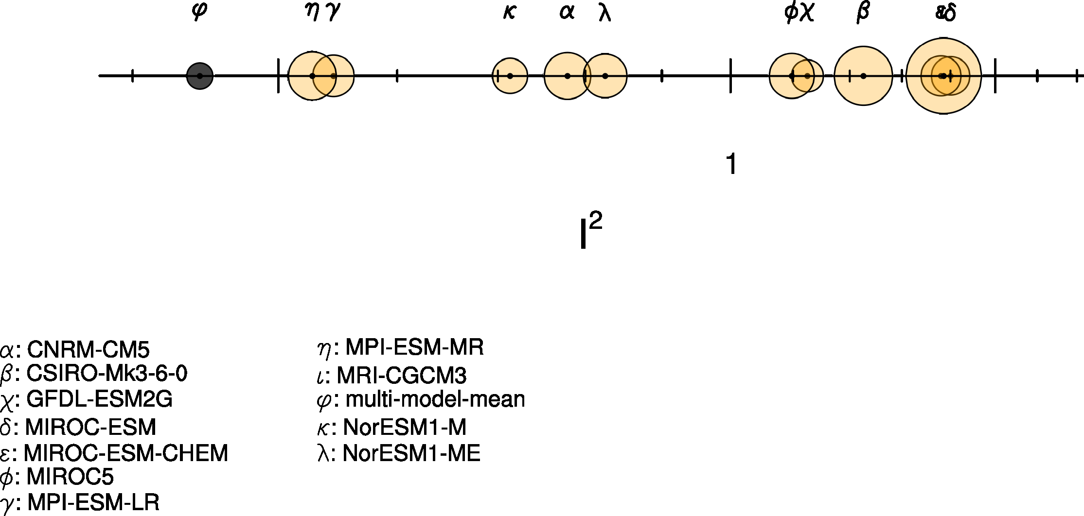
Fig. 87 Performance index I² for individual models (circles). Circle sizes indicate the length of the 95% confidence intervals. The black circle indicates the I² of the multi-model mean (similar to Reichler and Kim (2008), Figure 1).