16. Ozone and associated climate impacts
16.1. Overview
This namelist, implemented into the ESMValTool to evaluate atmospheric chemistry and the climate impact of stratospheric ozone changes, reproduces selected plots from Eyring et al. (2013), i.e. their figs. 1, 2, 4, 6, 7, 10, and 11. These include calculation of the zonally averaged seasonal cycle of total ozone columns (Figure 16.1), time series of the total ozone averaged over given regions (Figure 16.2), climatological mean tropospheric ozone columns (Figure 16.3), stratospheric ozone time series (Figure 16.4), differences in vertical ozone profiles between the 2090s and 2000s (Figure 16.5), trends in annual mean ozone, temperature, and jet position (Figure 16.6), and trend relationships between ozone and temperature and jet position (Figure 16.7).
16.2. Available namelists and diagnostics
Namelists are stored in nml/
- namelist_eyring13jgr.xml
Diagnostics are stored in diag_scripts/
- eyring13jgr_fig01.ncl: calculates seasonal cycles of zonally averaged total ozone columns.
- eyring13jgr_fig02.ncl: time series of area-weighted total ozone from 1960-2005 for the annual mean averaged over the global domain (90°S-90°N), Tropics (25°S-25°N), northern mid-latitudes (35°N-60°N), southern mid-latitudes (35°S-60°S), and the March and October mean averaged over the Arctic (60°N-90°N) and the Antarctic (60°S-90°S).
- eyring13jgr_fig04.ncl: climatological annual mean tropospheric ozone columns (geographical distribution).
- eyring13jgr_fig06.ncl: 1980 baseline-adjusted stratospheric column ozone time series from 1960-2100.
- eyring13jgr_fig07.ncl: differences in vertically resolved ozone between the 2090s and 2000s for the annual mean averaged over the global domain (90°S-90°N), Tropics (25°S-25°N), northern mid-latitudes (35°N-60°N), southern mid-latitudes (35°S-60°S), and the March and October mean averaged over the Arctic (60°N-90°N) and the Antarctic (60°S-90°S).
- eyring13jgr_fig10.ncl: trends in annual mean near-global (82.5°S-82.5°N) ozone at 50 hPa and temperature at 100 hPa, September-October-November-December (SOND) ozone at 50 hPa over Antarctica (60°S-90°S), October-November-December-January (ONDJ) temperature at 100 hPa over Antarctica (60°S-90°S), DJF SH jet position at 850 hPa, and DJF upper tropospheric tropical (30°S-30°N) temperatures at 250 hPa. The trends are calculated over 1979-2005 for the past and over 2006-2050 for the future.
- eyring13jgr_fig11.ncl: trend relationship between annual mean near-global (82.5°S-82.5°N) ozone at 50 hPa and temperature at 100 hPa, SOND ozone at 50 hPa and ONDJ temperature at 100 hPa over Antarctica (60°S-90°S), SOND ozone at 50 hPa and DJF jet position at 850 hPa; and DJF 250 hPa tropical (30°S-30°N) temperatures and DJF jet position at 850 hPa. The trends are calculated over 1979-2005 for the past and over 2006-2050 for the future.
16.3. User settings
User setting files (cfg files) are stored in nml/cfg_eyring13jgr
eyring13jgr_fig01.ncl
diag_script_info attributes
- rgb_file: path + filename of color table (e.g., “diag_scripts/lib/ncl/rgb/eyring_toz.rgb”)
- styleset: style set (“DEFAULT”, “CMIP5”)
- font: overrides default font (e.g., 21 ; see www.ncl.ucar.edu/Document/Graphics/Resources/tx.shtml#txFont)
- range_option: 0 = as in nml, 1 = overlapping time period
- lbLabelBarOn: plot a label bar (True, False)
- e13fig01_ = “True”
- e13fig01_list_chem_mod: list of models in the group “chem” (array of strings, default = (/”All”/))
- e13fig01_list_chem_mod_string: plotting label for group “chem”, e.g., “CMIP5”
- e13fig01_list_nochem_mod: list of models in the group “nochem” (array of strings, default = (/”“/))
- e13fig01_list_nochem_mod_string: plotting label for group “nochem”, e.g., “NoChem”
- e13fig01_diff_ref: name of reference model for difference plots, e.g., “NIWA”
eyring13jgr_fig02.ncl
diag_script_info attributes
- e13fig02_latrange: min. and max. latitude of the regions (n-element array of 2-element pairs, e.g., (/(/-90,90/), (/-90,-60/)/)); one pair of latitudes is required for each season (see below)
- styleset: style set (“DEFAULT”, “CMIP5”)
- e13fig02_season: seasons (n-element array of strings, “ANN”, “JAN”, “FEB”, “MAR”, “DJF”, “SON”, etc.)
- e13fig02_XMin: min. x-values (start years) for plotting (n-element array, e.g., (/1960., 1960./)); array is required to have the same number of elements as “seasons” (see above)
- e13fig02_XMax: max. x-values (end years) for plotting (n-element array, e.g., (/2005., 2005./)); array is required to have the same number of elements as “seasons” (see above)
- e13fig02_YMin: min. y-values for plotting (n-element array, e.g., (/260., 150./)); array is required to have the same number of elements as “seasons” (see above)
- e13fig02_YMax: max. y-values for plotting (n-element array, e.g., (/340.,500./)); array is required to have the same number of elements as “seasons” (see above)
- e13fig02_legend: plot legend (string, e.g., “True”)
- e13fig02_legend_MMM: include multi model mean in legend (string, e.g., “False”)
- list_chem_mod: list of models in the group “chem” (array of strings, default = (/”All”/)
- list_nochem_mod: list of models in the group “nochem” (array of strings, default = (/”None”/))
eyring13jgr_fig04.ncl
diag_script_info attributes
- styleset: style set (“DEFAULT”, “CMIP5”)
- font: overrides default font (e.g., 21 ; see www.ncl.ucar.edu/Document/Graphics/Resources/tx.shtml#txFont)
- range_option: 0 = as in nml, 1 = overlapping time period
- lbLabelBarOn: plot a label bar (True, False)
- e13fig04_ = “True”
- e13fig04_list_chem_mod: list of models in the group “chem” (array of strings, default = (/”All”/))
- e13fig04_list_chem_mod_string: plotting label for group “chem”, e.g., “CMIP5”
- e13fig04_list_nochem_mod: list of models in the group “nochem” (array of strings, default = (/”“/))
- e13fig04_list_nochem_mod_string: plotting label for group “nochem”, e.g., “NoChem”
- e13fig04_diff_ref: name of reference model for difference plots, e.g., “AURA-MLS-OMI”
- mpProjection: map projection, optional (e.g., “CylindricalEquidistant”) (see http://www.ncl.ucar.edu/Document/Graphics/Resources/mp.shtml#mpProjection for available projections)
eyring13jgr_fig06.ncl
diag_script_info attributes
- e13fig06_latrange: min. and max. latitude of the regions (n-element array of 2-element pairs, e.g., (/(/-90,90/), (/-90,-60/)/)); one pair of latitudes is required for each season (see below)
- styleset: style set (“DEFAULT”, “CMIP5”)
- e13fig06_season: seasons (n-element array of strings, “ANN”, “JAN”, “FEB”, “MAR”, “DJF”, “SON”, etc.)
- e13fig06_baseline_adj: do baseline adjustment (string: “True”, “False”)
- e13fig06_baseline: year for baseline adjustment (e.g., 1980)
- e13fig06_mod_plot: “MMT” = plot of the MultiModel mean of each scenario and selection “list_chem_mod” and “list_nochem_mod”; “IMT” = plot of each single model trend; “RAW” = plot of each model as raw data
- e13fig06_mod_plot_CI: plot confidence interval (string: “True”, “False”); for e13fig06_mod_plot = “MMT” only!
- e13fig06_mod_plot_PI: plot prediction interval (string: “True”, “False”); for e13fig06_mod_plot = “MMT” only!
- e13fig06_XMin: min. x-values (start years) for plotting (n-element array, e.g., (/1960., 1960./)); array is required to have the same number of elements as “seasons” (see above)
- 13fig06_XMax: max. x-values (end years) for plotting (n-element array, e.g., (/2010., 2010./)); array is required to have the same number of elements as “seasons” (see above)
- e13fig06_YMin: min. y-values for plotting (n-element array, e.g., (/260., 150./)); array is required to have the same number of elements as “seasons” (see above)
- e13fig06_YMax: max. y-values for plotting (n-element array, e.g., (/330., 500./)); array is required to have the same number of elements as “seasons” (see above)
- list_chem_mod: list of models in the group “chem” (array of strings, default = (/”All”/)
- list_nochem_mod: list of models in the group “nochem” (array of strings, default = (/”None”/))
- e13fig06_labels_exp_esp: specify experiment name (string: “True”, “False”); only if e13fig06_mod_plot = “IMT” or “RAW”!
eyring13jgr_fig07.ncl
diag_script_info attributes
- e13fig06_latrange: min. and max. latitude of the regions (n-element array of 2-element pairs, e.g., (/(/-90,90/), (/-90,-60/)/)); one pair of latitudes is required for each season (see below)
- styleset: style set (“DEFAULT”, “CMIP5”)
- e13fig07_season: seasons (n-element array of strings, “ANN”, “JAN”, “FEB”, “MAR”, “DJF”, “SON”, etc.)
- e13fig07_period1: start and end year of “period1” (= 2000s), e.g., (/2000., 2009/)
- e13fig07_period2: start and end year of “period2” (= 2090s), e.g., (/2090., 2099/)
- e13fig07_XMin: min. x-values for plotting (n-element array, e.g., (/-2., -2./)); array is required to have the same number of elements as “seasons” (see above)
- 13fig07_XMax: max. x-values for plotting (n-element array, e.g., (/2., 12./)); array is required to have the same number of elements as “seasons” (see above)
- list_chem_mod: list of models in the group “chem” (array of strings, default = (/”All”))
- list_nochem_mod: list of models in the group “nochem” (array of strings, default = (/”None”/))
eyring13jgr_fig10.ncl
diag_script_info attributes
- e13fig10_latrange: min. and max. latitude of the regions (n-element array of 2-element pairs, e.g., (/(/-30, 30/)/)); one pair of latitudes is required for each season (see below)
- styleset: style set (“DEFAULT”, “CMIP5”)
- e13fig10_season: seasons (n-element array of strings, e.g., “ANN”, “JAN”, “FEB”, “MAR”, “DJF”, “SON”, etc.)
- e13fig10_lev: vertical level (in hPa)
- plot_number: string used for plot labeling / sub-figure (e.g., “(a)”)
- list_chem_mod: list of models in the group “chem” (array of strings, default = (/”All”/)
- list_nochem_mod: list of models in the group “nochem” (array of strings, default = (/”None”/))
eyring13jgr_fig11.ncl
diag_script_info attributes
- styleset: style set (“DEFAULT”, “CMIP5”)
- e13fig11_V0_units: unit label for “variable 0” (x-axis) (string)
- e13fig11_V1_units: unit label for “variable 1” (y-axis) (string)
- e13fig11_V0_latrange: min. and max. latitude of the region for “variable 0”
- e13fig11_V1_latrange: min. and max. latitude of the region for “variable 1”
- e13fig11_V0_season: season for “variable 0” (e.g., “yearly”)
- e13fig11_V1_season: season for “variable 1” (e.g., “yearly”)
- e13fig10_V0_lev: vertical level (in hPa) for “variable 0”
- e13fig10_V1_lev: vertical level (in hPa) for “variable 1”
- plot_number: string used for plot labeling / sub-figure (e.g., “(a)”)
- e13fig11_XMin: min. x-value for plotting
- e13fig11_XMax: max. x-value for plotting
- e13fig11_YMin: min. y-value for plotting
- e13fig11_YMax: max. y-value for plotting
- list_chem_mod: list of models in the group “chem” (array of strings, default = empty)
- list_nochem_mod: list of models in the group “nochem” (array of strings, default = empty)
16.4. Variables
- tro3 (atmos, monthly mean, longitude latitude lev time)
- ta (atmos, monthly mean, longitude latitude lev time)
- ua (atmos, monthly mean, longitude latitude lev time)
16.5. Observations and reformat scripts
Total column ozone (toz): NIWA (Bodeker et al., 2005)
Reformat script: reformat_scripts/obs/reformat_obs_NIWA.ncl
Tropospheric column ozone (tropoz): MLS/OMI (Ziemke et al., 2006)
Reformat script: reformat_scripts/obs/reformat_obs_AURA-MLS-OMI.ncl
16.6. References
- Eyring, V., J. M. Arblaster, I. Cionni, J. Sedlacek, J. Perlwitz, P. J. Young, S. Bekki, D. Bergmann, P. Cameron-Smith, W. J. Collins, G. Faluvegi, K.-D. Gottschaldt, L. W. Horowitz, D. E. Kinnison, J.-F. Lamarque, D. R. Marsh, D. Saint-Martin, D. T. Shindell, K. Sudo, S. Szopa, and S. Watanabe, Long-term ozone changes and associated climate impacts in CMIP5 simulations, J. Geophys. Res. Atmos., 118, doi: 10.1002/jgrd.50316, 2013.
16.7. Example plots
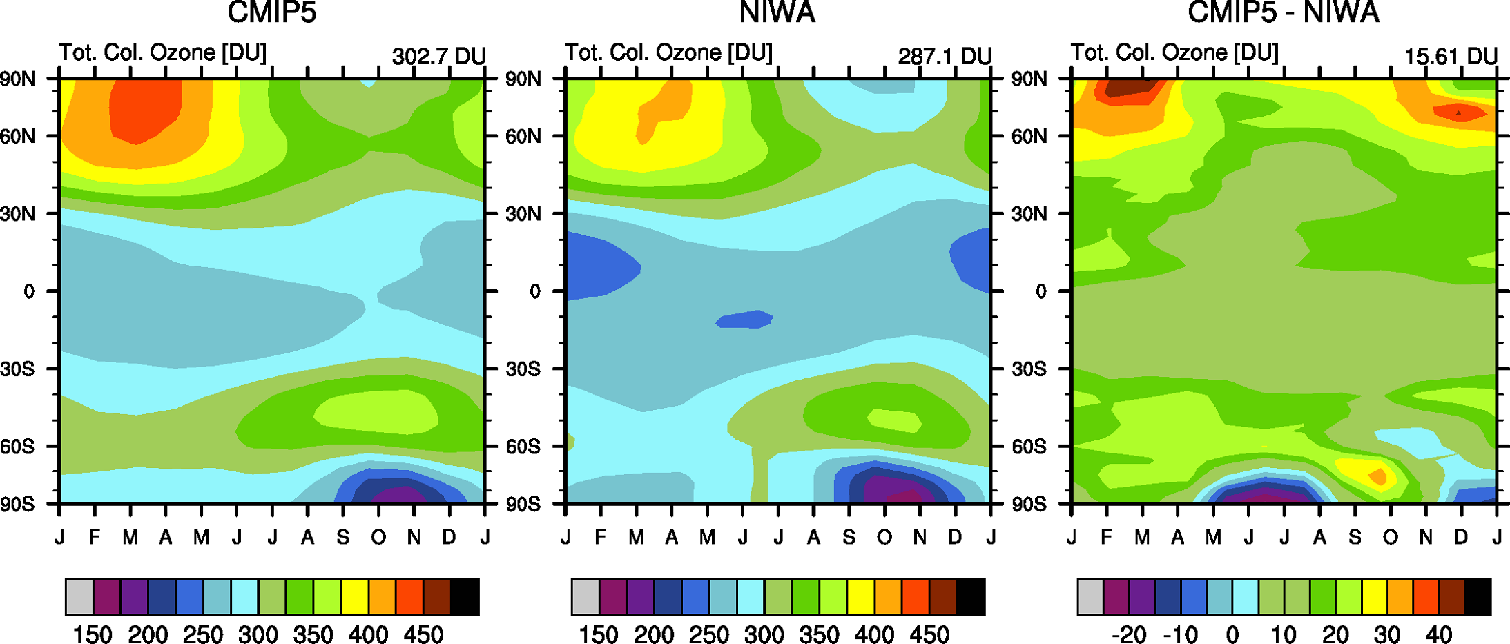
Figure 16.1 Produced with “eyring13jgr_fig01.ncl”.
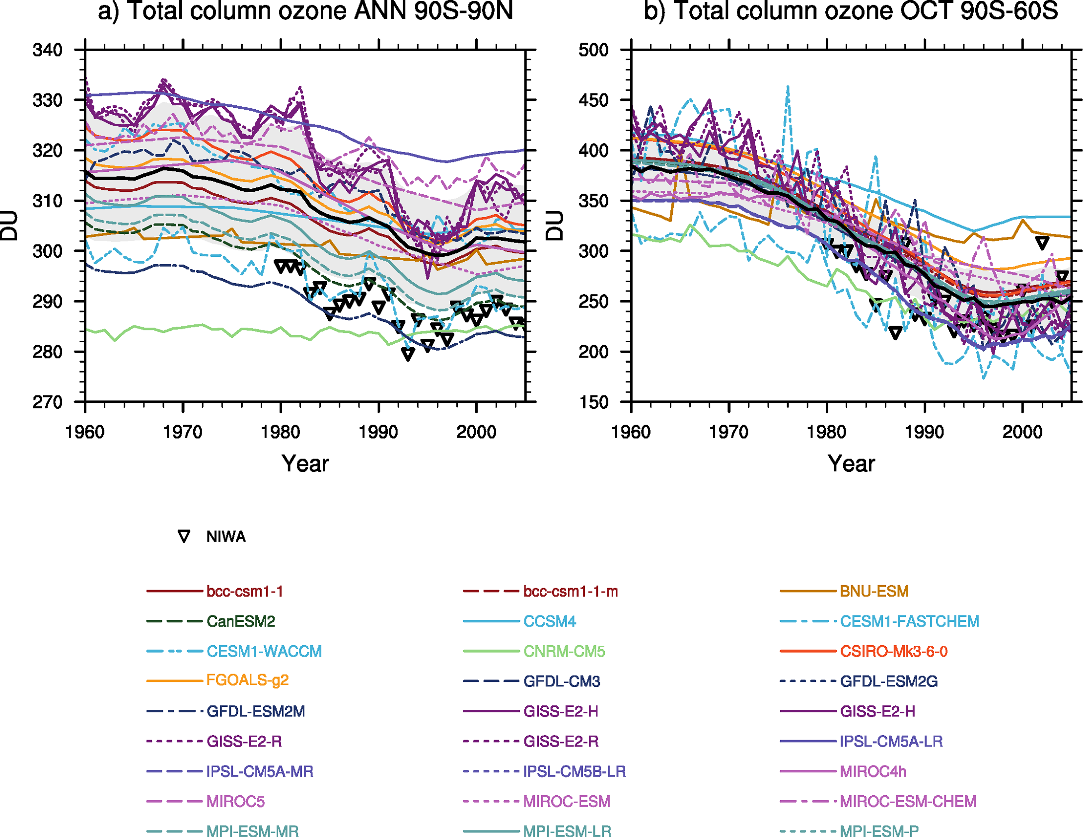
Figure 16.2 Produced with “eyring13jgr_fig02.ncl”.
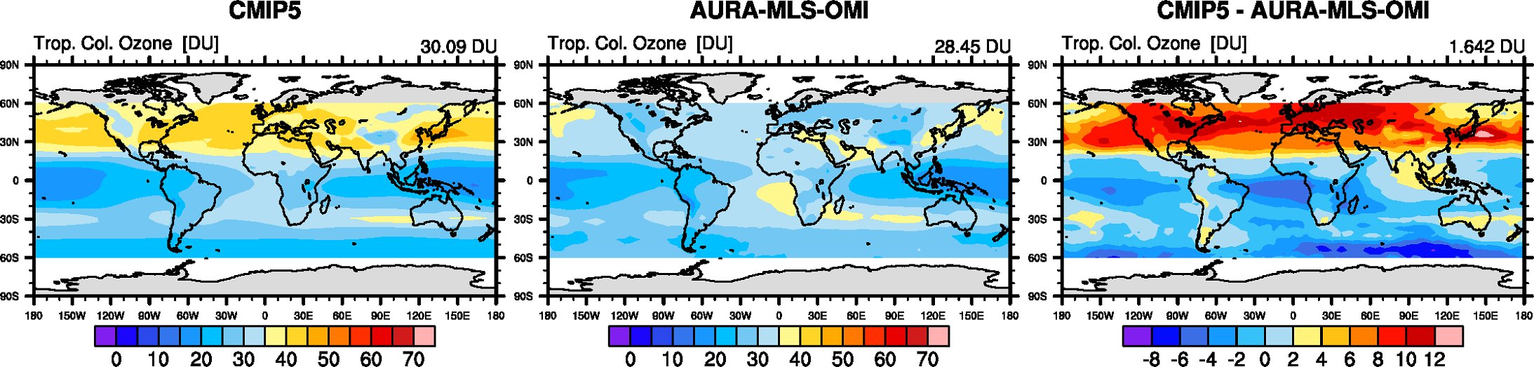
Figure 16.3 Produced with “eyring13jgr_fig04.ncl”.
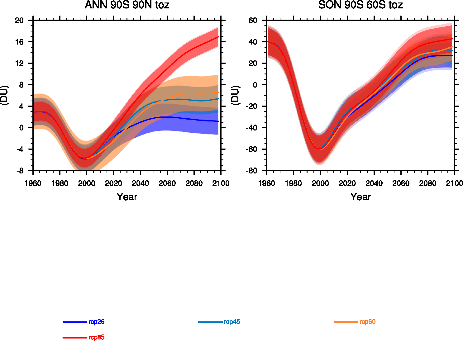
Figure 16.4 Produced with “eyring13jgr_fig06.ncl”.
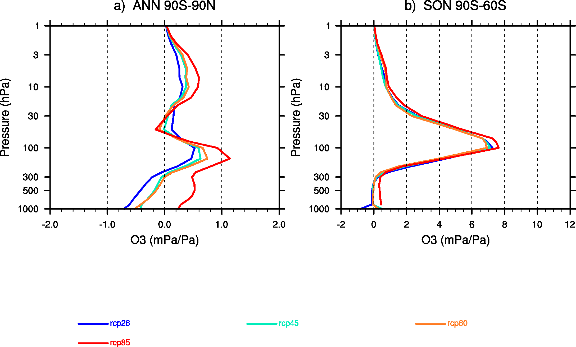
Figure 16.5 Produced with “eyring13jgr_fig07.ncl”.
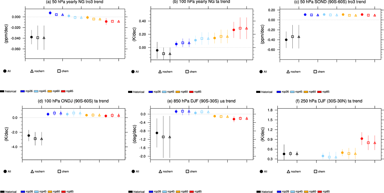
Figure 16.6 Produced with “eyring13jgr_fig10.ncl”.
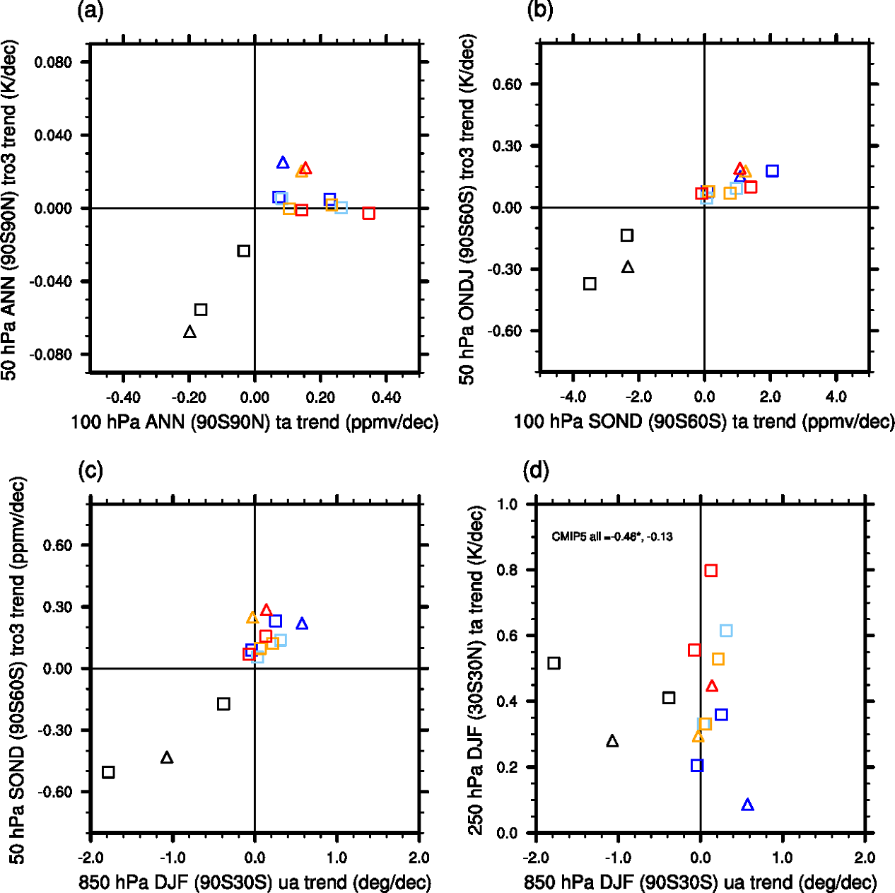
Figure 16.7 Produced with “eyring13_jgr_fig11.ncl”