24. Standardized Precipitation Index (SPI)
24.1. Overview
For each month, the precipitation over the preceding TIMESCALE months, x, is summed. Then a two-parameter Gamma distribution of cumulative probability, Gammaα,β, is fitted to the strictly positive TIMESCALE month sums, such that the probability of a non-zero precipitation sum being below a certain value x corresponds to Gammaα,β(x). We estimate shape parameter α and scale parameter β with a maximum likelihood approach. If the estimation does not converge, α and β are approximated using empirical relations (Bordi et al., 2001). Accounting for TIMESCALE month periods of no precipitation, occurring at a frequency q, the total cumulative probability distribution of a precipitation sum below x, H(x), becomes H(x) = q + (1 - q) * Gammaα,β(x). In the last step, a precipitation sum x is assigned to its corresponding Standardized Precipitation Index (SPI) value by computing the quantile qN(0,1) of the standard normal distribution at probability H(x). The SPI of a precipitation sum x, thus, corresponds to the quantile of the standard normal distribution which is assigned by preserving the probability of the original precipitation sum, H(x).
24.2. Available namelists and diagnostics
Namelists are stored in nml/
- namelist_SPI.xml
Diagnostics are stored in diag_scripts/
- SPI.r
24.3. User settings
User setting files (cfg files) are stored in nml/cfg_SPI/
- SPR.r
- begin.ref.year: first year of the reference period
- end.ref.year: last year of the reference period
- timescale: valid values are 3, 6 and 12 months
- seasons: “ann”, “djf”, “mam”, “jja”, “son”
- spi_colorbar_max: color bar range (= -spi_colorbar_max … +spi_colorbar_max)
- my.colors: colors for contour plot, e.g., colorRampPalette(c(“brown”, “orange”, “white”, “lightblue”, “blue”))
- png_width: width of png image
- png_height: height of png image
- png_units: units of png dimensions (“px” = pixels, “in” = inches, “cm” = centimeters, “mm” = millimeters)
- png_pointsize: the default size of plotted text in points (1/72 inch)
- png_bg: background color, e.g., “white”
24.4. Variables
- pr (atmos, monthly mean, longitude latitude time)
24.5. Observations and reformat scripts
Note: (1) obs4mips data can be used directly without any preprocessing; (2) see headers of reformat scripts for non-obs4mips data for download instructions.
24.6. References
A very good explanation of SPI
- Lloyd-Hughes, B. and Saunders, M. A. (2002), A drought climatology for Europe. Int. J. Climatol., 22, 1571-1592. doi: 10.1002/joc.846.
Other standard SPI references
- Guttman, N. B. (1999), ACCEPTING THE STANDARDIZED PRECIPITATION INDEX: A CALCULATION ALGORITHM. JAWRA Journal of the American Water Resources Association, 35, 311-322. doi: 10.1111/j.1752-1688.1999.tb03592.x.
- McKee, T. B., N. J. Doesken, and J. Kliest, 1993: The relationship of drought frequency and duration to time scales. In Proceedings of the 8th Conference of Applied Climatology, 17-22 January, Anaheim, CA. American Meterological Society, Boston, MA. 179-184.
- McKee, T. B, N. J. Doesken, and J. Kliest, 1995: Drought Monitoring with Multiple Time Scales. 9th AMS Conference on Applied Climatology, 15-20 January 1995, Dallas, Texas.
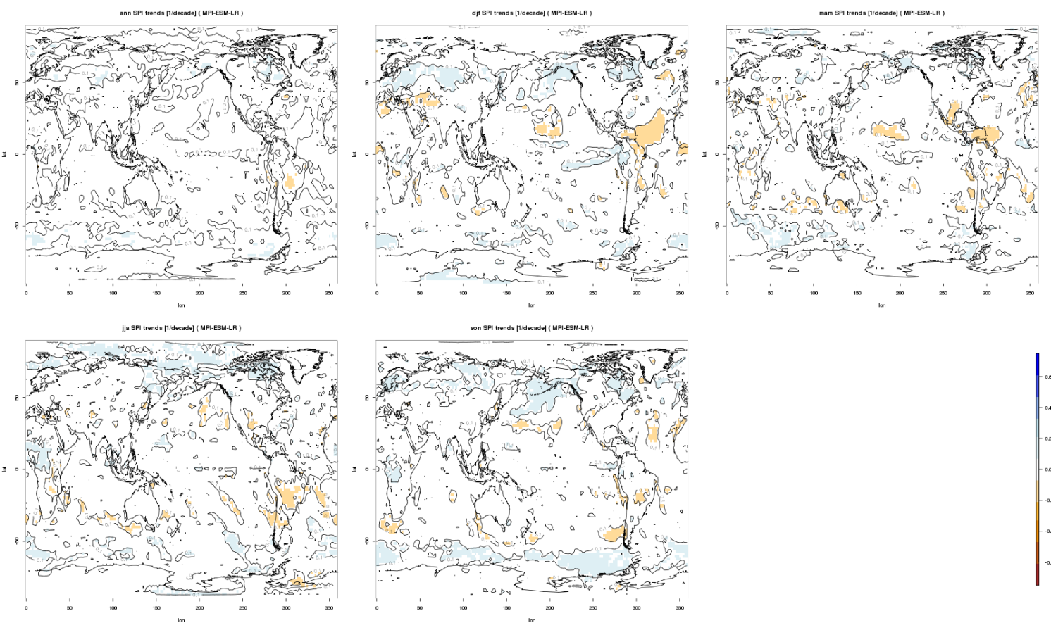
24.7. Example plots